\[\newcommand{\norm}[1]{\left\lVert#1\right\rVert}\]

Part 1: Fit a Neural Field to a 2D Image.

For this part, we create a neural network that takes a 2D coordinate as input and output an RGB value. We’ll use this to model a function mapping the pixel coordinate of a picture and its RGB value.

Ultimately, we’d like for the network to remember this image:

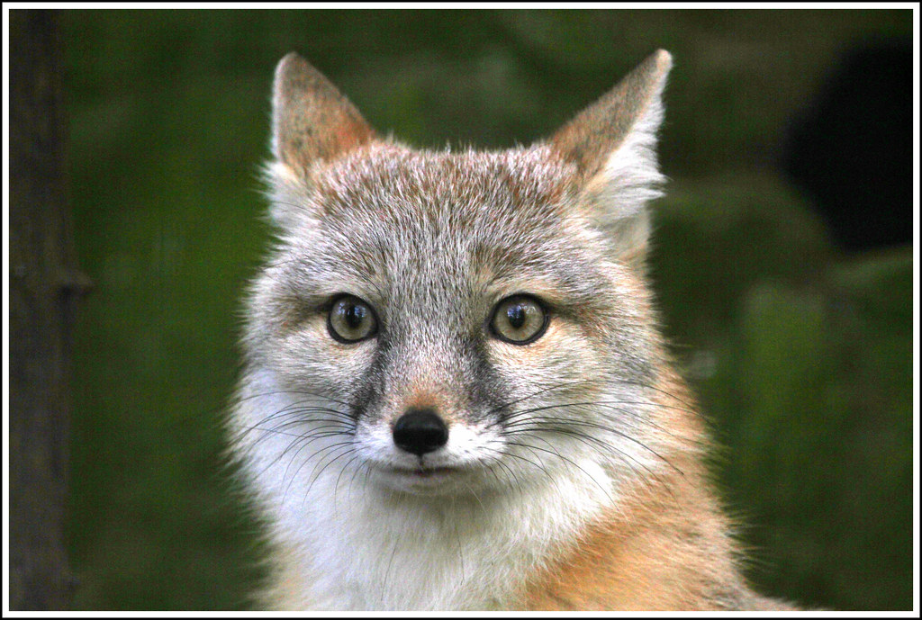
To enable the network to learn higher frequencies better, we’ll use a sinusoidal positional encoding. In particular, we generate the following features from a single spatial coordinate:

\[PE(x) = \{x, sin(2^0\pi x), cos(2^0\pi x), sin(2^1\pi x), cos(2^1\pi x), ..., sin(2^{L-1}\pi x), cos(2^{L-1}\pi x)\}\]

where $L$ is the highest frequency value.

We use the architecture recommeneded:

Optimizing the network with a 10k batch size for 3000 iterations with the Adam optimizer (learning rate = 1e-3), we observe the following loss and PSNR curve.

Here are some reconstructions at various iterations:

At iteration=20

at iteration=100

at iteration=500

and at iteration=1500

We also tried to increase the length of the positional encoding to see if our network could learn finer details better. There was not a perceptible difference:

With L = 10

With L = 30

We try the same procedure with an image of Maria Callas (L=30, Adam optimizer with lr=1e-3) during her Medea performance.

Original: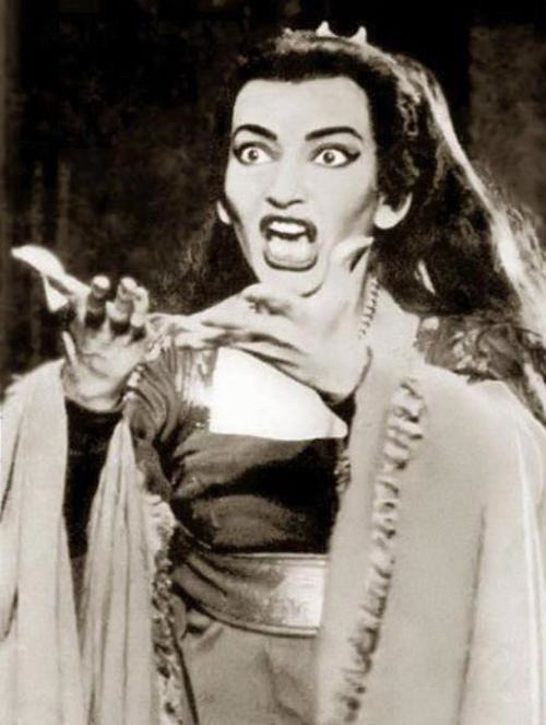

Reconstruction at it=100:

Reconstruction at it=300:

Reconstruction at it=1500:

Reconstruction at it=3000:

Loss (log-scale):

PSNR:

Part 2: NeRF

To convert fom a camera coordinate $x_c$ to world coordinate $x_w$ we simply perform a multiplication with the $c2w$ matrix. To convert from pixel $(u, v)$ to camera coordinate, we simply multiply both sides of the following equation with $K^{-1}$

\[\begin{align} s \begin{bmatrix} u \\ v \\ 1 \end{bmatrix} = \mathbf{K} \begin{bmatrix} x_c \\ y_c \\ z_c \end{bmatrix} \end{align}\]

To convert from a pixel $(u, v)$ to a ray going from the camera’s COP to said pixel, we first compute the camera origin with $\begin{align} r_o = -\mathbf{R}_{3\times3}^{-1}\mathbf{t} \end{align}$ where $\mathbf{t}$ is the 3x1 last column of the c2w matrix. Then the direction vector is: $\begin{align} \mathbf{r}_d = \frac{\mathbf{X_w} - \mathbf{r}_o}{||\mathbf{X_w} - \mathbf{r}_o||_2} \end{align}$ where $\mathbf{X}_w$ is the point (in world coordinate) at depth s=1 from the camera.

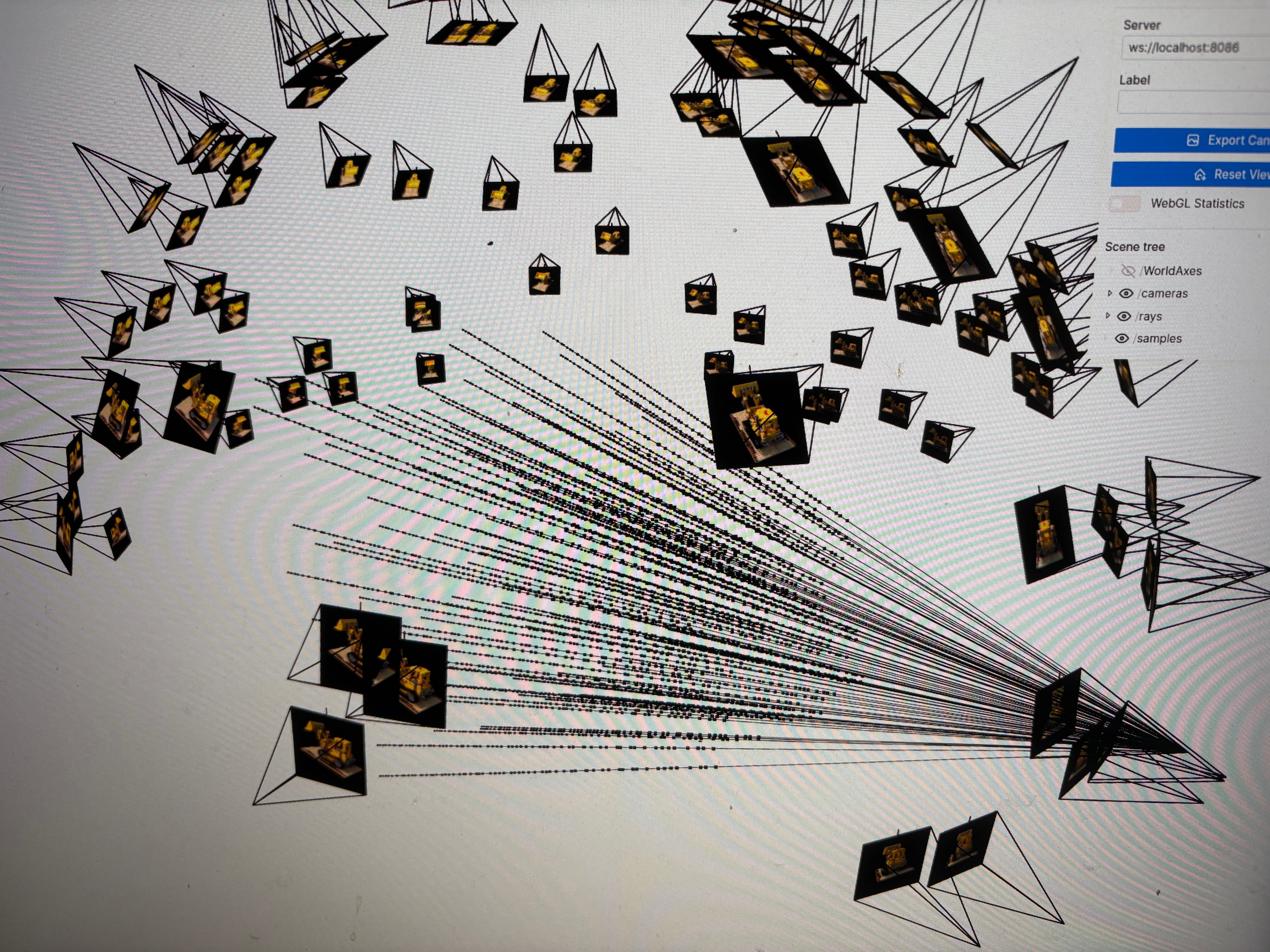
To sample N rays from the dataset, we chose to sample $N / DatasetSize$ rays from each image. To calculate the world coordinates of the sapmle points along each ray, we simply use the equation $\mathbf{x} = \mathbf{R}_o + \mathbf{R}_d * t$. We also add some noise to $t$ to prevent overfitting.

Here’s a visualization of our sampling rays:

Here’s our network architecture:

We used $L=10$ for $x$ and $L=4$ for $r_d$. We trained for 8000 iterations with Adam optimizer (lr=5e-4), n_samples=192 and was able to achieve an PSNR between 23 and 24.

Here are the validation PSNR and Loss curve:

Here are a few samples along the trainig process (the right is the reference picture):

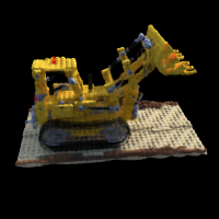
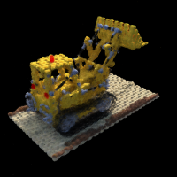
Here are the comparisons between the validation picture and our reconstruction at 8000 iterations:

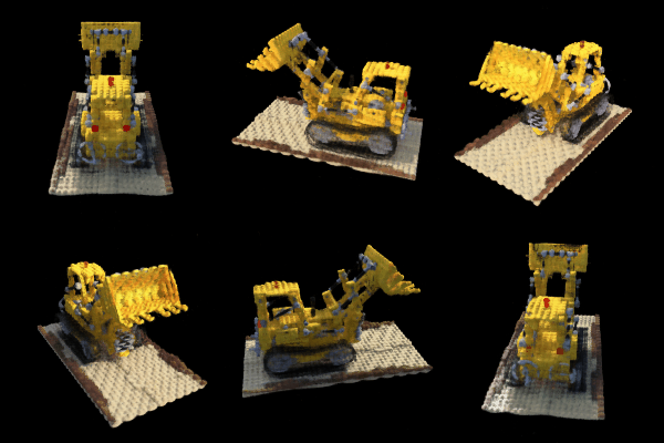
Here are some frames in the rotating gif:

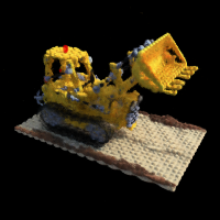
Here’s a gif:

Bells & Whistles

For B&W, we altered the volrend function to yield a different background:

To achieve this, we first identified the pixels whose rays contain samples that are all identically black. Once we’ve identified the background pixels, we simply assign one of the sample point our desired background color and proceed as before.