Project 3: Face Morphing
Part 1: Define correspondences
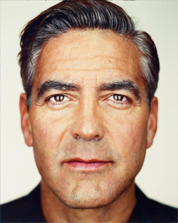
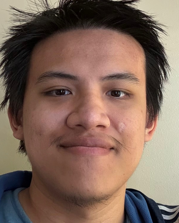
In this part, I’ll attempt to create a morph between a picture of myself and George.
| George | Me |
|---|---|
 |
 |
To start, we’ll first have to use the provided tool to define 2 corresponding point clouds (i.e. a set of (x, y) coordinates) for each image. Here are the results with the point clouds and Delauney triangulation inplace:
| George | Me |
|---|---|
Part 2: Computing the “mean” face
Next, To align our faces together, I wrote computeAffine(pts1, pts2) which outputs a matrix that transforms each point (out of 3) in pts1 to pts2, where pts1 and pts2 are points in a triangle belonging to our triangulation. I did this in 2 steps. First, create matrix $T_1$ that takes each points in the standard basis $(0, 0), (1, 0), (0, 1)$ to $A, B, C \in $ pts1. A quick inspection tells us:
From this, $T_1^{-1}$ can be computed, provided that the 3 points in pts1 aren’t colinear. Next, create matrix $T_2$ that transform the standard basis into each point $A’, B’, C’$ in pts2.
Once this is done, our transform matrix will simply be $T_2T_1^{-1}$.
Now we can compute the inverse warp for each triangle in the triangulation.
Let $A, B, C$ be the vertices of a particular triangle in our destination image and $A’, B’, C’$ be the corresponding vertices in our source image. Our transformation matrix is then $T = $ computeAffine({A, B, C}, {A', B', C'}).
Let $P$ (for polygon) be the set of points contained in the boundary of $A, B, C$ in our destination. The corresponding set of points in the source image would then be $T(P)$, where the transformation $T$ is applied to each point in $P$.
Since some of these points in $T(P)$ will not lie on integer coordinates, we’ll have to use interpolation. I found RectBivariateSpline worked well.
All that’s left is to loop over each triangle and assign each pixel in the destination the corresponding pixel value in the source image: dest[pt] = interpolated_source[T @ pt].
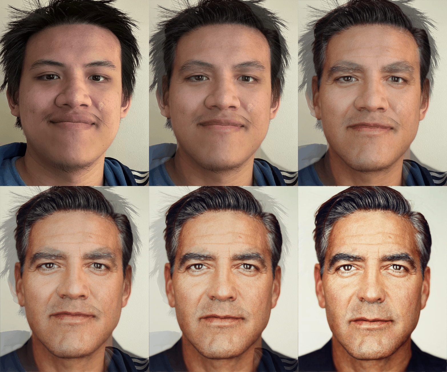
With this, I morphed my and George’s image to the “average point cloud” (i.e. the average face shape, which could be computed by simply taking the average of corresponding points from each image) and computed the average. Here’s the results:
The first row is our original faces. The second is our faces morphed into the “middle” face shape. The final row is the cross-dissolve average.
Part 3: The Morph Sequence
Now we can compute the “morph sequence” easily. Let $t \in [0, 1]$, and $cloud_0, cloud_1$ be the set of corresponding points in image 1 and 2 respectively. Also, let tri be the triangulation of the mean point cloud (i.e. (cloud0 + cloud1) / 2).
At time step $t$, we can compute the “weighted point cloud” by avg_cloud = (1 - t) * cloud_0 + t * cloud_1. We can then compute the “morphosis” of image 1 and image 2 to this weighted average using the proceture in the previous part. The morphed image at time step $t$ can be achieved by simply using cross dissolve: morphed = (1 - t) * im1_to_avg + t * im2_to_mid.
Now we can simply vary $t$ and collect the resulting pictures in a gif.
Here’s the result of me morphing to George.

Part 4: Mean Face of a population.
In this part, we’ll compute the average male face from the “Danes” dataset. Here are some male faces constituting the average from said dataset:
In order not to have too much “smoothing”, we’ll first align all the faces to a common face shape. The most natural common face shape is just the average of the face shapes. Here’s the result of aligning each face to the average face shape:
With this, we can simply take average (pixel-wise) over all the aligned faces. Here’s the result of doing that:
Note that without first aligning the face shape, we’d get a very blurry result:
For fun (and credit), I also morphed my face into the average geometry and vice versa. Since the average face shape was taken over the non-smiling faces, note the joy dropping out of my face in the me2average morph :(
| Me2Average | Avg2Me |
|---|---|
Part 5: Caricatures
For this part, we’ll use PCA to create an exaggerated face shape. The point cloud for each face consists of 62 points. We can treat each point cloud as a point in a high-dimensional space of dimension $62*2=124$. Let $X$ then be the samples matrix (each of the $32$ rows is a $124$ dimensional vector representing the point cloud).
Consider the SVD of the sample matrix: $X = U\Sigma V^T$. If $x_i$ and $u_i$ are the $i$-th row of $X$ and $U$, respectively, then we have $x_i = u_i \Sigma V^T$. This suggests that the rows of $X$ are the rows of $U$ under some linear transformation ($\Sigma V^T$ to be precise) and that the singular values in $\Sigma$ indicates the influence (i.e. importance) of each dimension in the row space of $U$. This means we can drop some relatively unimportant singular values.
Graphing the singular values, we see that keeping about 10 of them should be enough.
Now, we can simply project my face geometry into the PCA components, scale them, then revert them back into the point cloud and realign my face to the newly obtained point cloud. Here are the resulting geometries from scaling my PCA-components-projected face geometry by $1.5, 2,$ and $3$:
Here’s some more caricatures done on portraits from the Danes dataset: