Project 2: Frequencies
1. Fun with Filters.
1.1 Finite Difference Operator
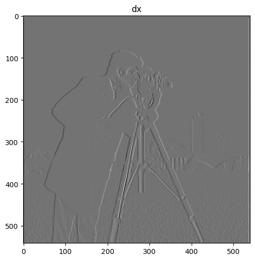
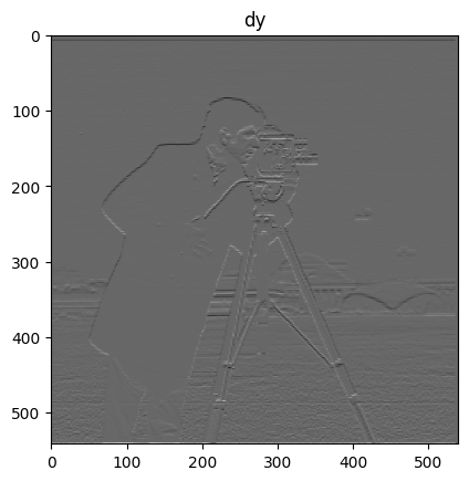
To compute the gradient image $\frac{\partial im}{\partial x}$ and $\frac{\partial im}{\partial y}$, we convolve the image with $D_x$ and $D_y$:
| $dx$ | $dy$ |
|---|---|
 |
 |
We compute the gradient magnitude by $\sqrt{\frac{\partial im}{\partial x}^{2} + \frac{\partial im}{\partial y}^{2}}$, which gives
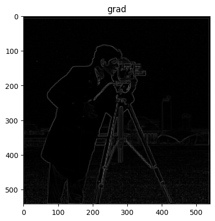
To pick an appropriate threshold for binarization, we look at the histogram of the gradient intensity:
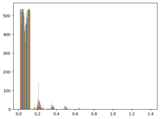
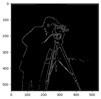
From the graph, we see setting a threshold greater than about 0.3 will exclude a lot of noises. So the binarized image ends up being grad > 0.3, which looks like:
1.2 Derivative of Gaussian (DoG).
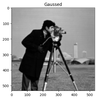
To get a better binarized image, we’ll first filter out the higher frequencies by convolving the image with a Gaussian filter. This gives:
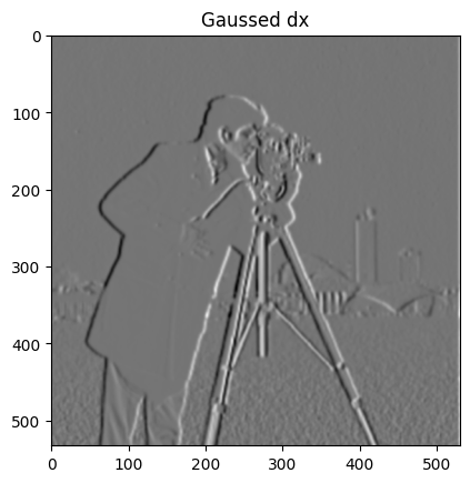
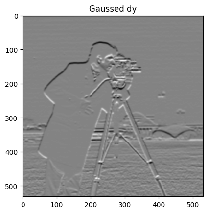
Taking the derivatives as the previous part yields:
| $dx$ | $dy$ |
|---|---|
 |
 |
The corresponding gradient magnitude is then:
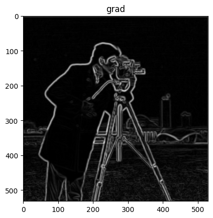
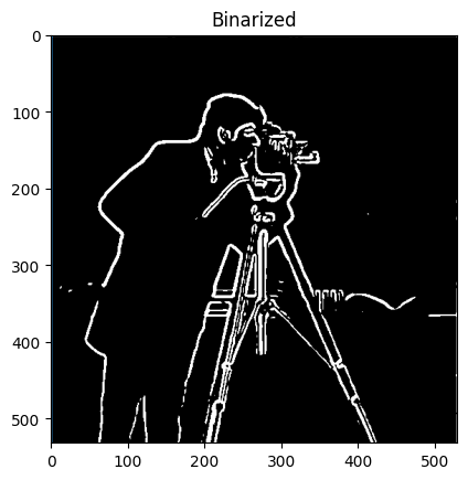
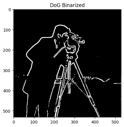
The edges look more pronounced and there is less noise than the previous part. We can similarly perform binarization to further reduce noise and highlight the relevant edges. So grad > 0.07 gives us:
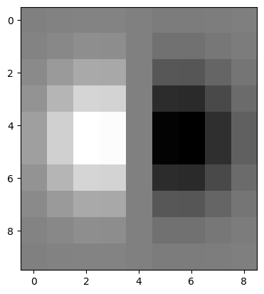
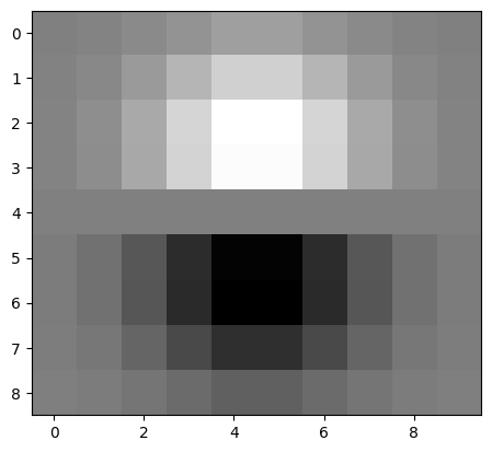
Since convolution is associative, we can convolve the image with the the derivative of the Gaussian instead. Mathematically, this means $(im * G) * D_x = im * (G * D_x)$. The derivatives of the Gaussian filter look as follows:
| $G * D_x$ | $G * D_y$ |
|---|---|
 |
 |
Convolving the image directly with this derivative of Gaussian and perform binarization gives us the same result:
2. Fun with Frequencies.
2.1 Image Sharpening.
We’ll try to achieve image sharpening by amplifying the higher frequencies. To do this, we convolve the image with a sharpening filter that amplifies the higher frequencies by a factor of $\alpha$. Mathematically, we want $im + \alpha(im - im * G) = im * e + \alpha\cdot im * e - \alpha\cdot im * G = im * ((1 + \alpha)e - \alpha \cdot G)$.
Here’s a sample of the sharpening filter that we’ve just derived. Notice the very slight depression in value around the peak!
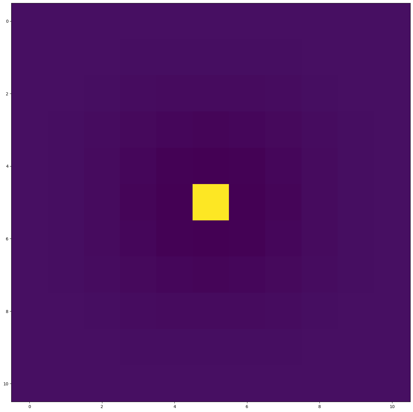
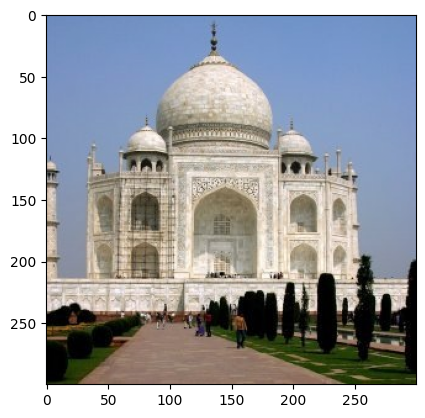
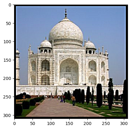
Convolving taj.jpg with said filter gives as the desired sharpening effect:
| Before | After |
|---|---|
 |
 |
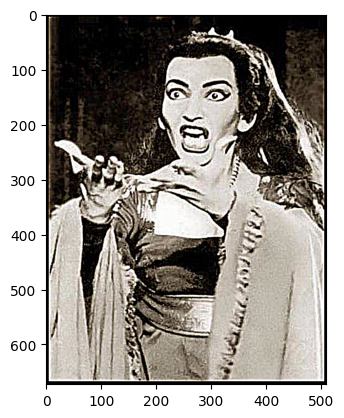
Here’s the sharpening effect on a photo of Maria Callas performing Medea with $\alpha=5.0$. We can finally see her glorious rage in 4k.
| Before | After |
|---|---|
 |
Now we sharpen the image taj, blur, then sharpen again. We can see that sharpening again doesn’t bring back all the details the original sharpened image had. This means bluring and sharpening are neither lossless processes nor inverses of one another.
2.2 Hybrid Images.
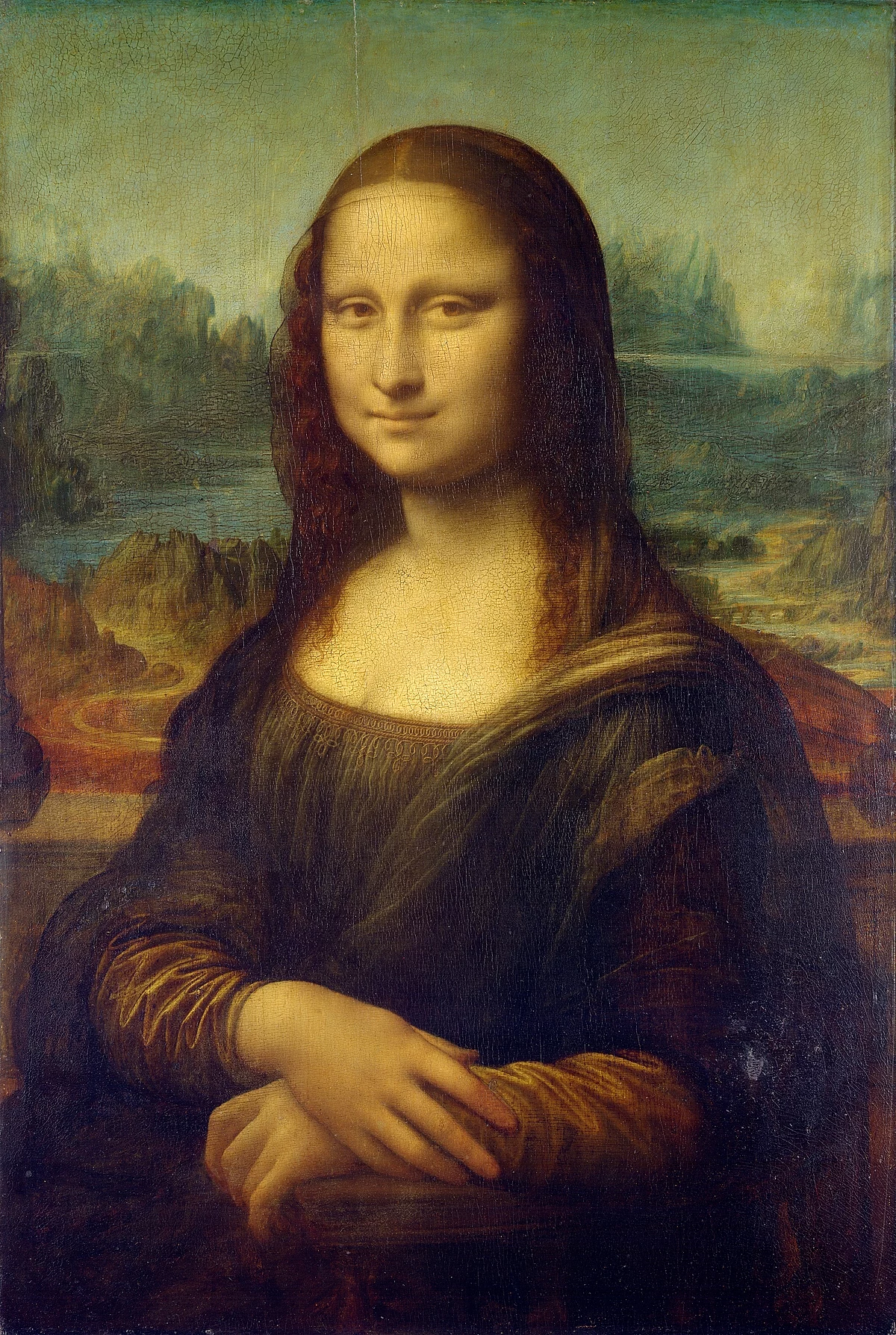
| Mona Lisa | Salvator Mundi |
|---|---|
 |
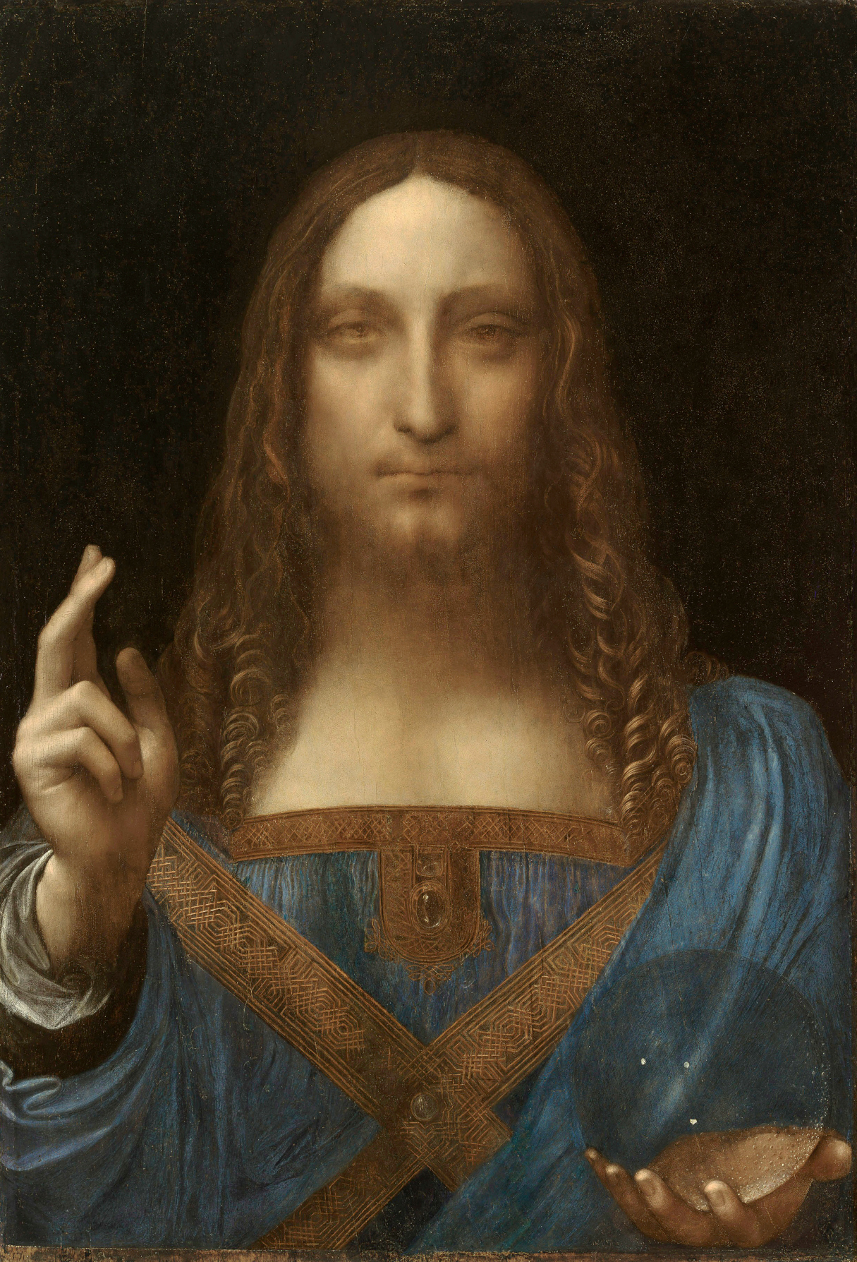 |
To illustrate, let’s blend the Mona Lisa and the Salvator Mundi (both famous paintings from Leonardo da Vinci). First, we’ll high-pass filter the Mona Lisa. We can do that by convolving Lisa with $e - G$ where $e$ is the unit impulse and $G$ is the low-pass Gaussian.
Here’s the highpass version of Mona Lisa, with the Fourier Magnitudes before and after the highpass filtering:
Next, we need to lowpass filter the Salvator Mundi. This is done by simply convolving the Mundi with a Gaussian. Here’s the lowpass Mundi, with the Fourier Magnitudes before and after. Notice how lowpass filtering attenuates the Fourier magnitudes at the corners.
To accentuate the effect, we choose to preserve color at the higher frequencies. After converting Mundi to greyscale and combine with Lisa we get:
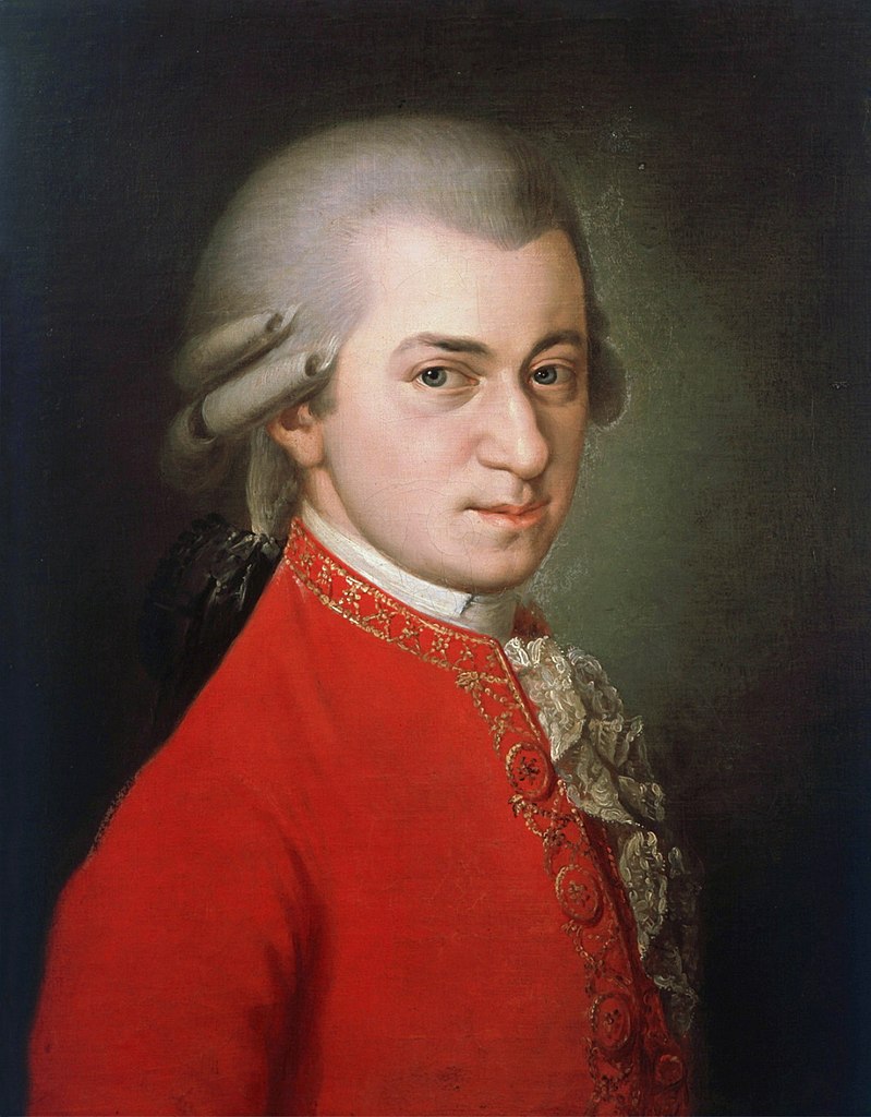
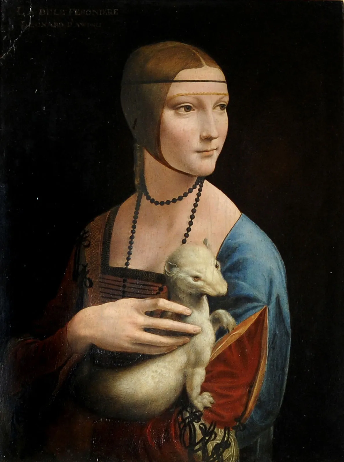
Here’s another hybrid image of a Mozart portrait and a Lady holding an Ermine:
| Mozart | Ermine Lady | Combined |
|---|---|---|
 |
 |
|
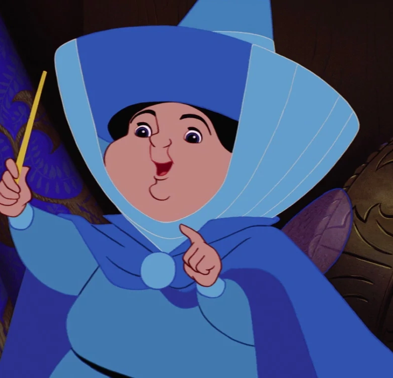
Lastly, here’s a hybrid of Maleficent and Merryweather (both from Sleeping Beauty). Notice the use of color at the high frequencies! Despite that, this example doesn’t work super well because the two characters are too different.
| Maleficent | Merryweather | Combined |
|---|---|---|
 |
 |
|
2.3 Laplacian Pyramid
A Laplacian Pyramid is a sequence of bandpass images constructed from the original image $I$ that captures high to low band of frequencies. Let $G_0 = I$ and $G_i = SubsampleBy2(GaussianFilter(G_{i-1}))$. Let $L_i = G_i - UpsampleBy2(G_{i-1})$. We call the sequence $L_i$ the Laplacian pyramid. At the lowest level, we simply let $L_N = G_N$. This allows us to write the following formula for the reconstruction of the original image (i.e. “collapsing” the pyramid): $G_0 = I = \sum_{k=0}^{N} L_k$.
To spline two images, we introduce a weighting function called region, which looks like this:
Let $L_i^{A}$ and $L_i^{B}$ be the Laplacian pyramid for the apple and orange image respectively. Let $G_k$ be the Gaussian pyramid for the region image. To spline together apple and orange, we simply construct a third Laplacian pyramid $L_k^{S} = G_k \cdot L_k^{A} + (1 - G_k) \cdot L_k^{B}$, then collapse the “spline” Laplacian pyramid to retrieve our spline image.
In the following picture, each row represents 3 terms from each level of the Laplacian pyramid: $G_i\cdot L_i^{A}$, $(1 - G_i)\cdot L_i^{B}$, and $L_k^{S}$. The last image shows the result when collapsing our Laplacian pyramid.
2.4 Laplacian Pyramid
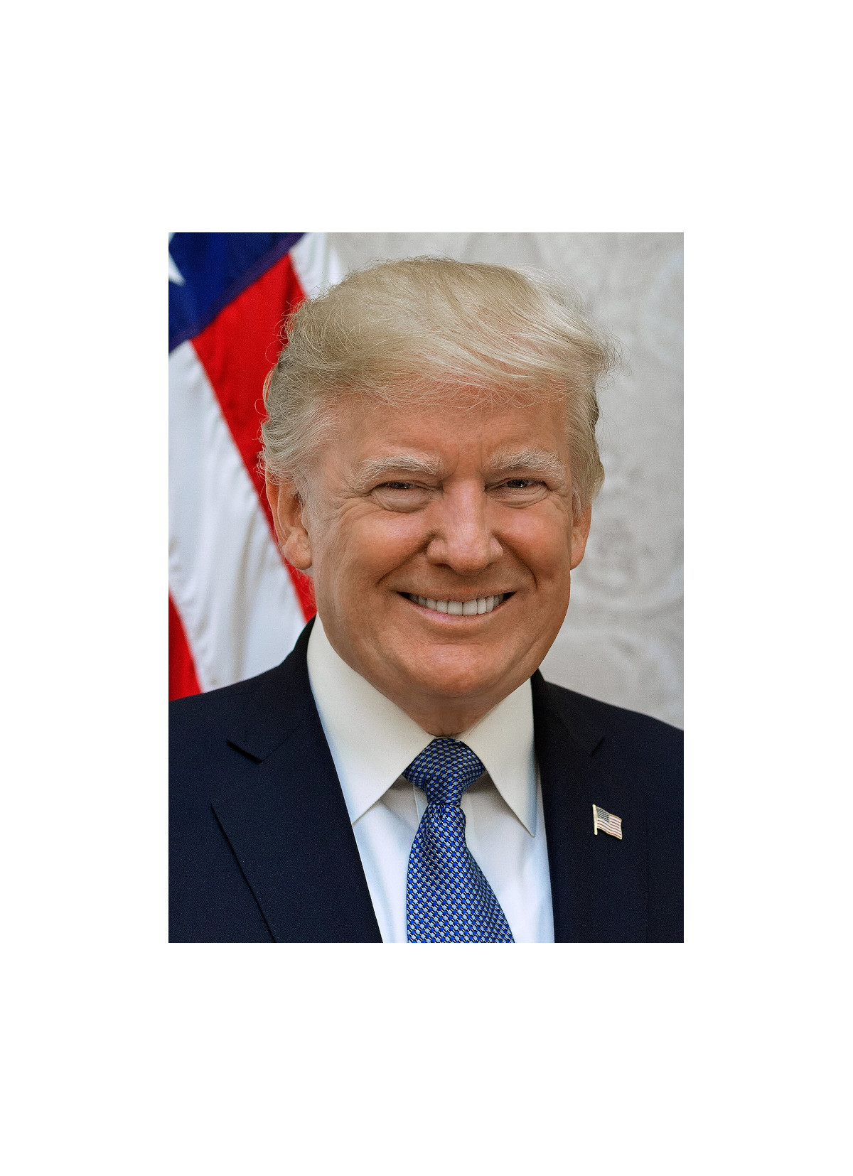
For an application of splining, let’s spline together a portrait or Kamala Harris and Donald Trump.
| Kamala Harris | Donald Trump | Combined |
|---|---|---|
 |
 |
|
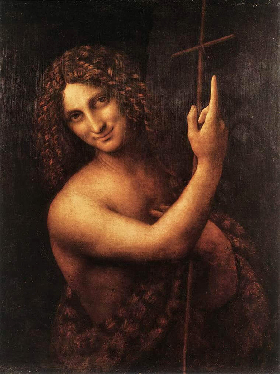
We can also do this with an irregular region function. For example, with this region mask, we can spline together the Mona Lisa and John The Baptist by Leonardo da Vinci.
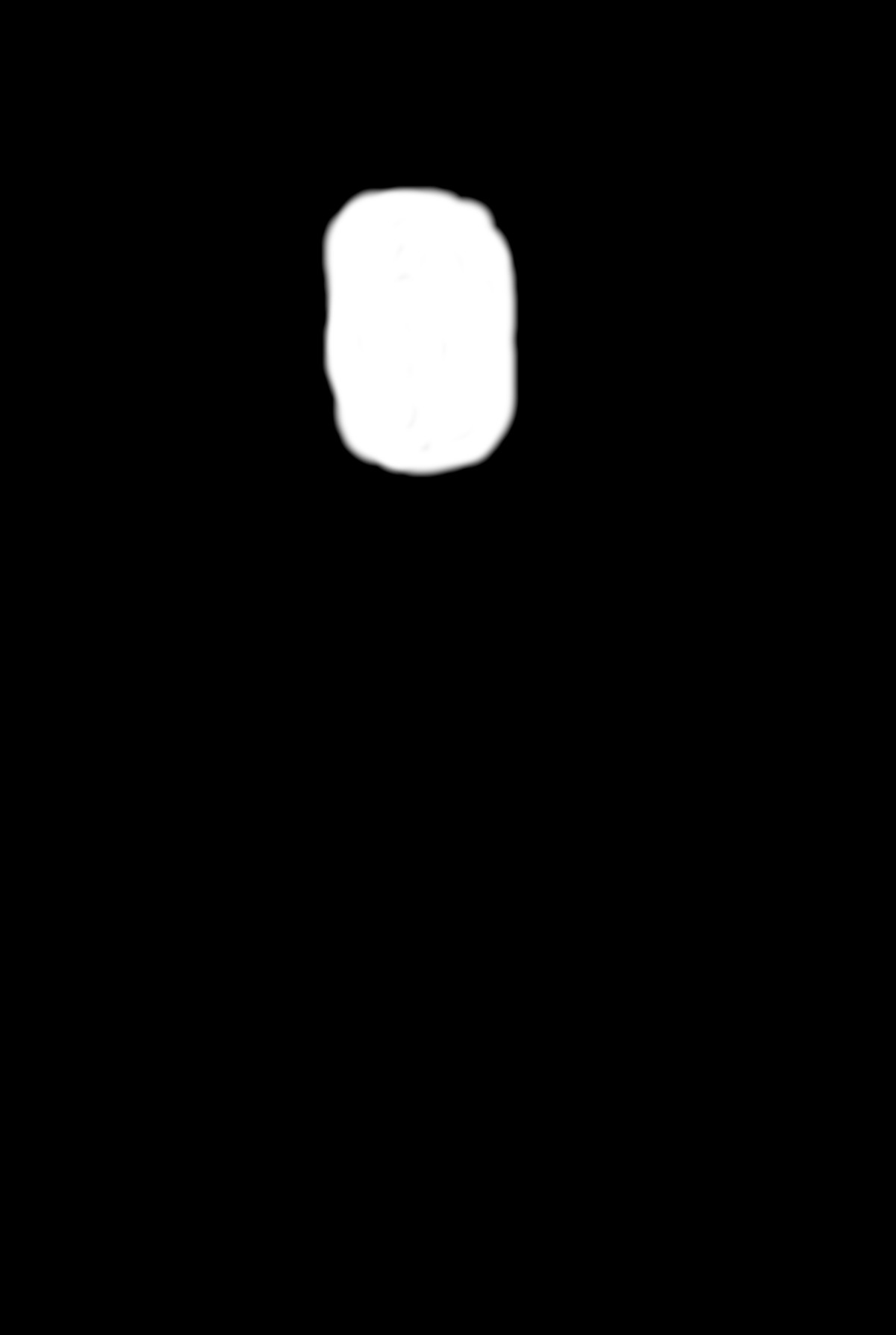
| Mona Lisa | John The Baptist | Combined |
|---|---|---|
 |
 |
|