Project 4: Mosaic

\[\newcommand{\norm}[1]{\left\lVert#1\right\rVert}\]

Part 1: Rectification

In this part, we’ll rectify a painting within another painting. Consider the following painting:

Suppose we now want to retrieve a more frontal view of the sub-painting on the bottom right. To do this, we’ll need to compute a projective transformation of the 4 key points (appeared as red circles in the picture) such that in the post-transform version, those 4 points appear as a rectangle.

Fact: The point $(x, y, z)$ and its projective-transformed version $(x’, y’, z’)$ are related in the following way, where $w$ is a constant.

\[\begin{bmatrix} a & b & c \\ d & e & f \\ g & h & 1 \end{bmatrix} \begin{bmatrix} x \\ y \\ 1 \end{bmatrix} = \begin{bmatrix} wx' \\ wy' \\ w \end{bmatrix}\]

We can then rewrite the equations as follows so that the unknowns are the coefficient of the matrix:

\[\begin{align*} \begin{cases} ax + by + c = wx' \\ dx + ey + f = wy' \\ gx + hy + 1 = w \end{cases} \\ \implies \begin{cases} ax + by + c = (gx + hy + 1) x' \\ dx + ey + f = (gx + hy + 1) y' \end{cases} \\ \implies \begin{cases} ax + by + c - gxx' - hyx' = x' \\ dx + ey + f - gxy' - hyy' = y' \end{cases} \\ \implies \begin{bmatrix} x & y & 1 & 0 & 0 & 0 & -xx' & -yx' \\ 0 & 0 & 0 & x & y & 1 & -xy' & -yy' \\ \end{bmatrix} \begin{bmatrix} a \\ b \\ c \\ d \\ e \\ f \\ g \\ h \end{bmatrix} = \begin{bmatrix} x' \\ y' \end{bmatrix} \end{align*}\]

Notice we can stack multiple correspondences $(x, y), (x’, y’)$ by simply extending the LHS matrix and the RHS column vector. Since there could be more correspondences than unknowns, we’ll simply use least squares to find the best fit.

We can then use inverse warping to find the resulting rectification. Doing that for the image above gives:

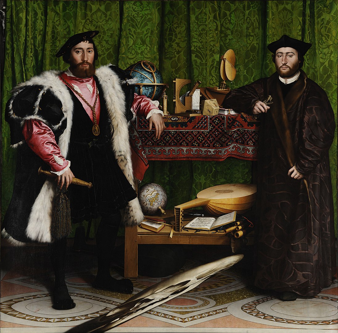
Here’s the result of rectifying the skull in “The Ambassadors”:

Part 2: Mosaic

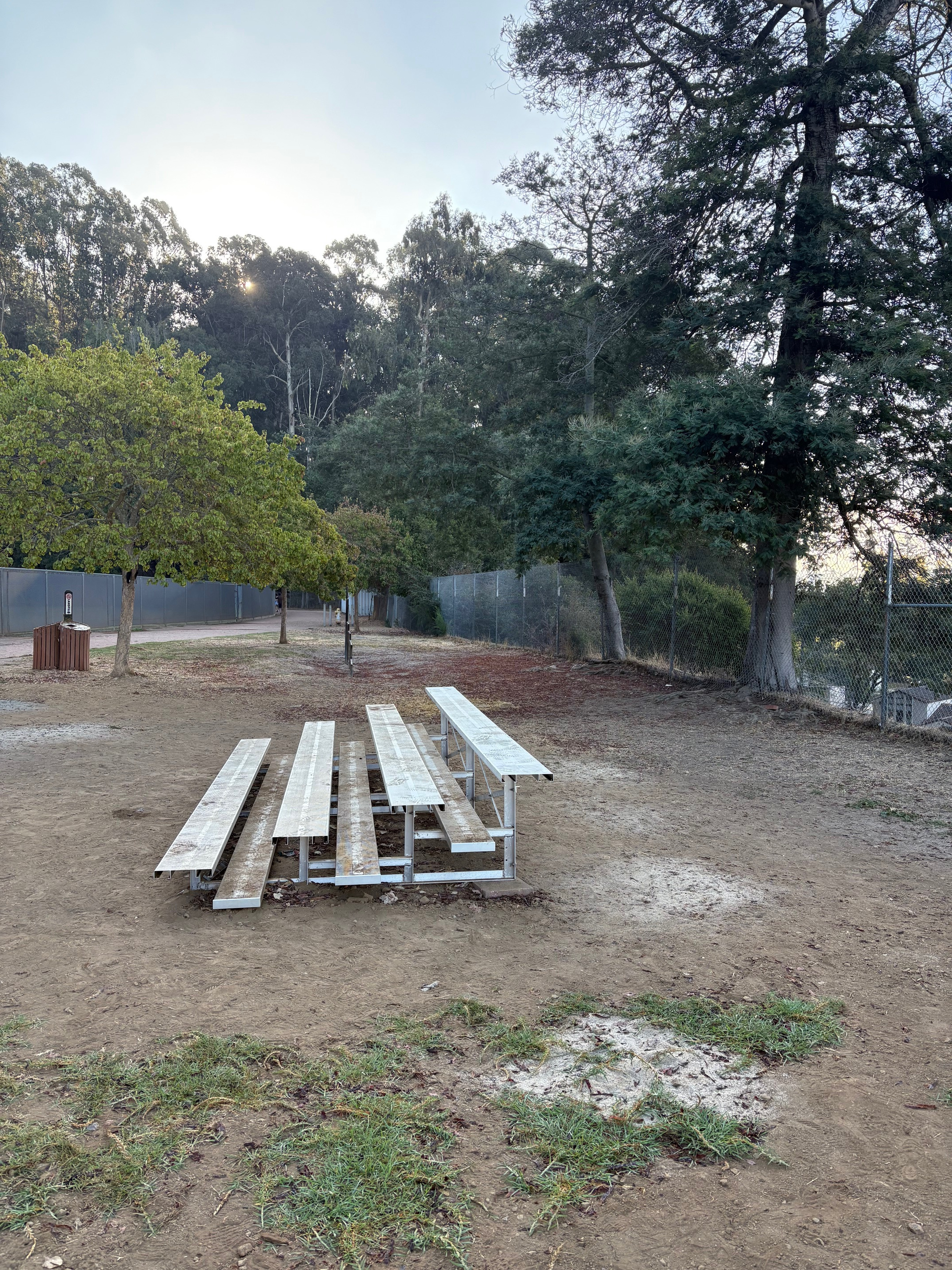
Suppose now we have two images taken from the same center-of-projection and we’d like to fuse them together.

Left	Right

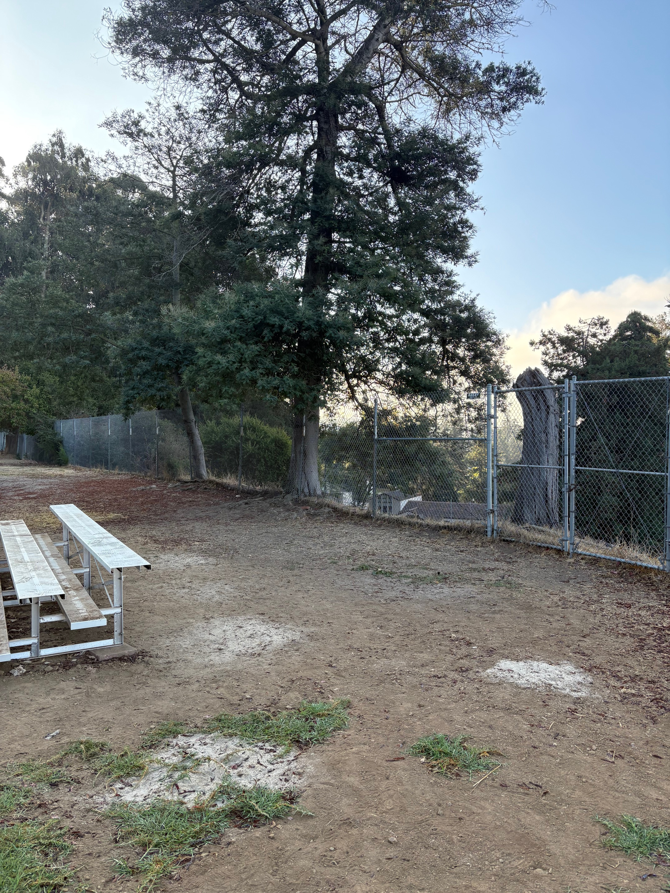We’d first need to define some correspondences:

Left	Right

Now we’ll just need to compute the homography that would transform the point cloud in the right image to the point cloud in the left image. Here’s what the projectively-transformed 2nd image looks like:

Left	Right

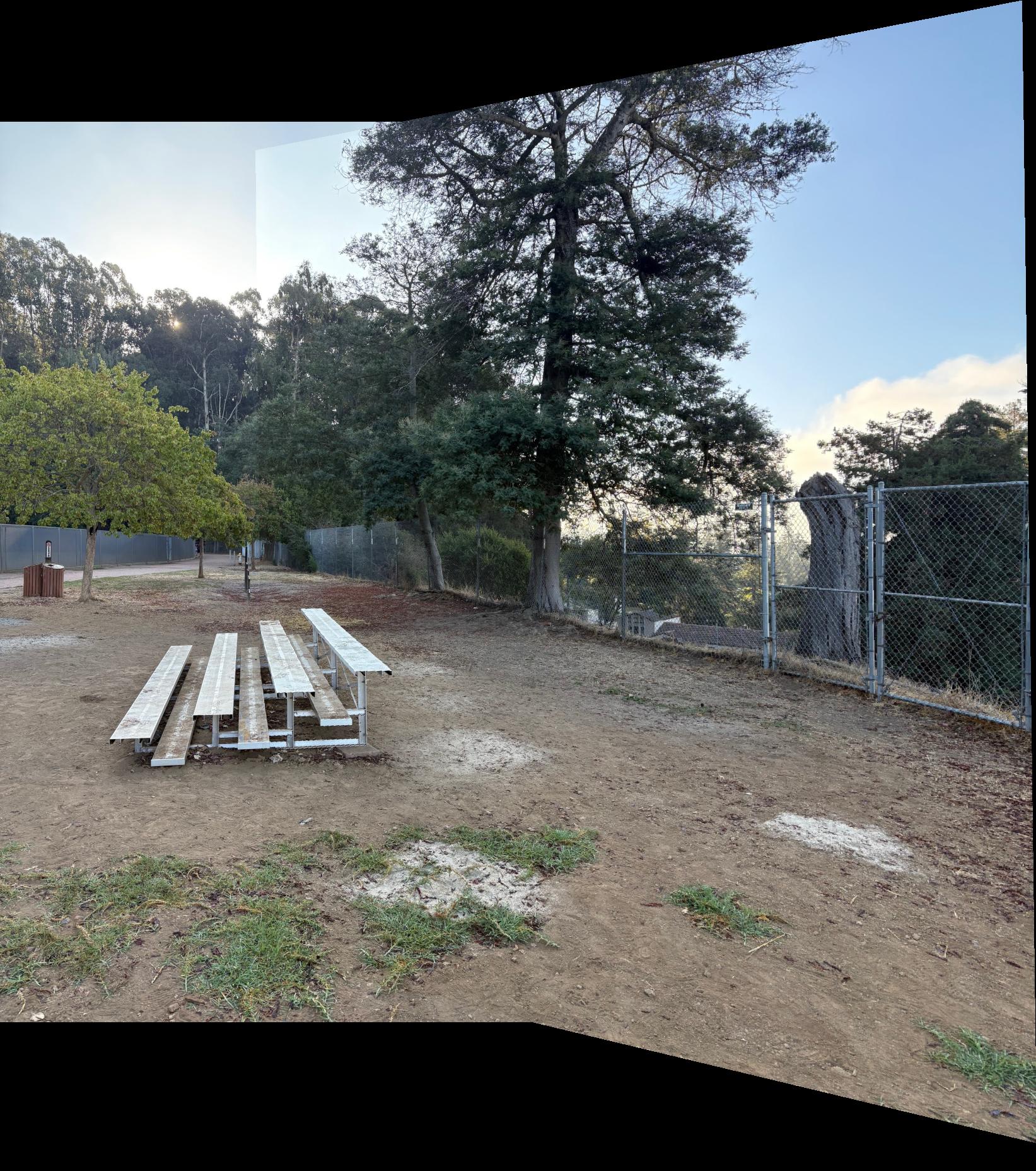
Finally, we just need to blend them together, which results in:

Part 3: Auto-Mosaic

To automate this process, we’ll first need to do feature detection. To that end, we’ll use the Harris corner detector on our original picture:

UnFeatured	Featured

Since there are too many features to be computationally efficient, we’ll remove some of them. If we simply take the points with the highest corner response, we’ll get:

This is not desirable since the points might be highly concentrated in one area but not as concentrated in the region where two images overlap. To combat this, we’ll use Adaptive Non-Maximal Suppression. This results in a more spread out point cloud. Here’s an example of ANMS with radius of 10:

Now, we extract an 8-by-8 feature descriptor at each point-of-interest by supsampling (with anti-aliasing) from a 40-by-40 window. We also normalized the mean and standard variance of the image.

We then use a K-D Tree to implement nearest-neighbor matching. Using Lowe’s trick with threshold set at 0.4, we found the following correspondences:

There are indeed good correspondences but it is clear from the picture that some outliers exist as well. To combat that, we’ll run RANSAC. Setting epsilon at 2 (pixels) and do 1000 rounds of iterations, we arrived at the following:

It’s clear that the bad outliers have been removed. Now, all that’s left is to create a mosaic using our earlier function. Doing so gives something that’s indistinguishably close to the mosaic obtained using manual correspondences:

Manual	Automatic

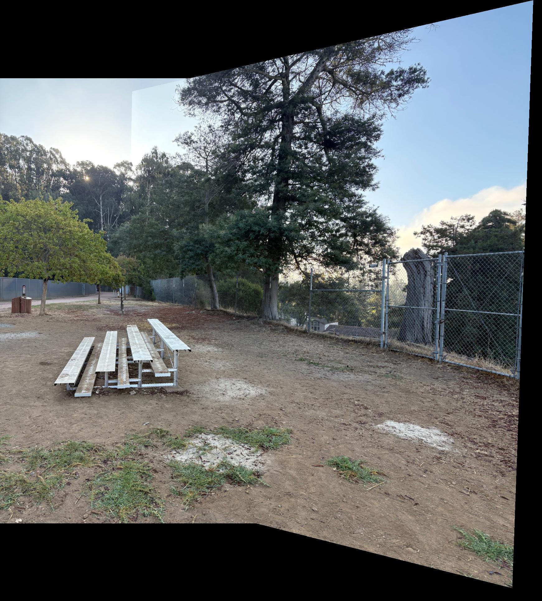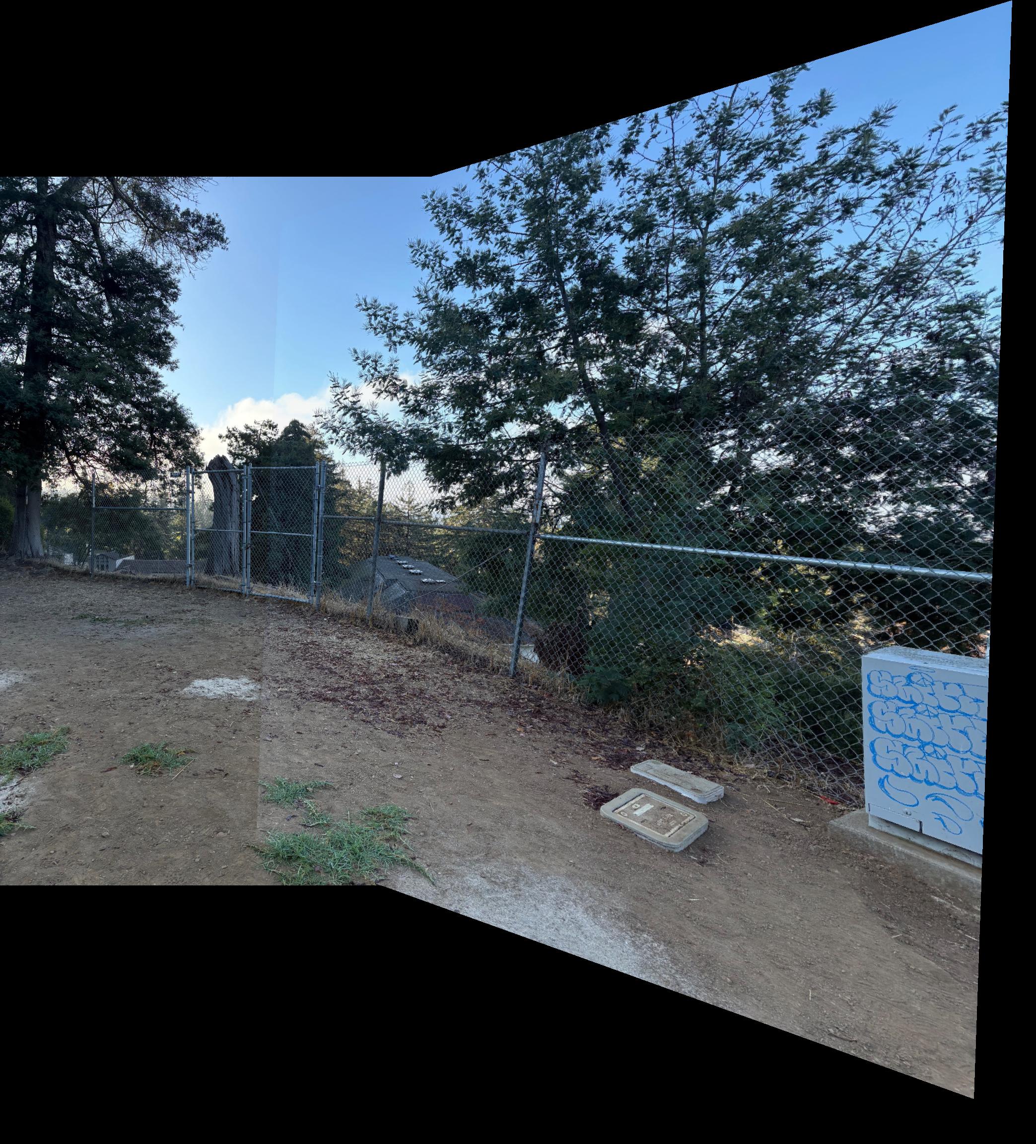
Here are 2 more mosaics that were obtain through our automated system:

1	2	3

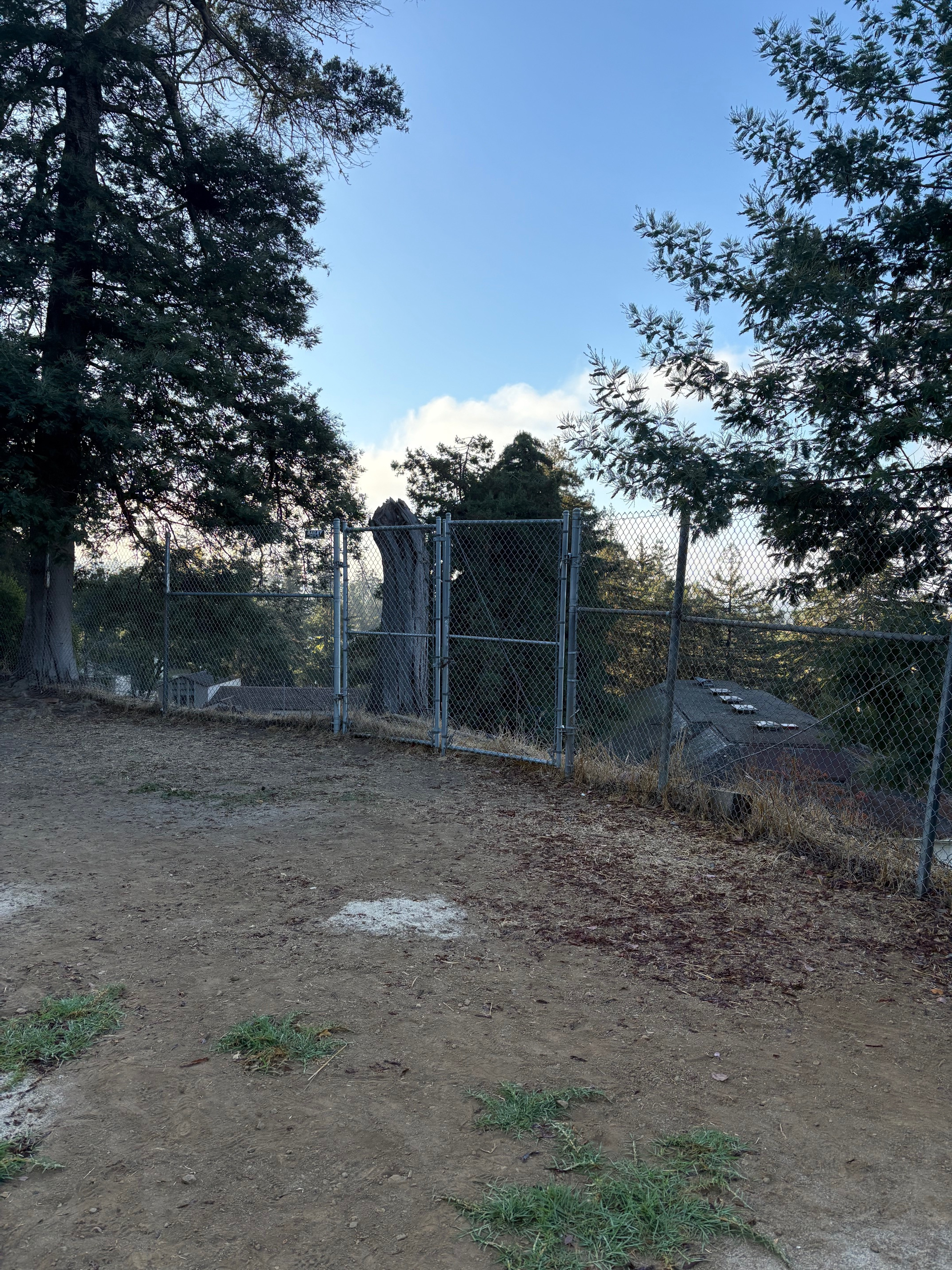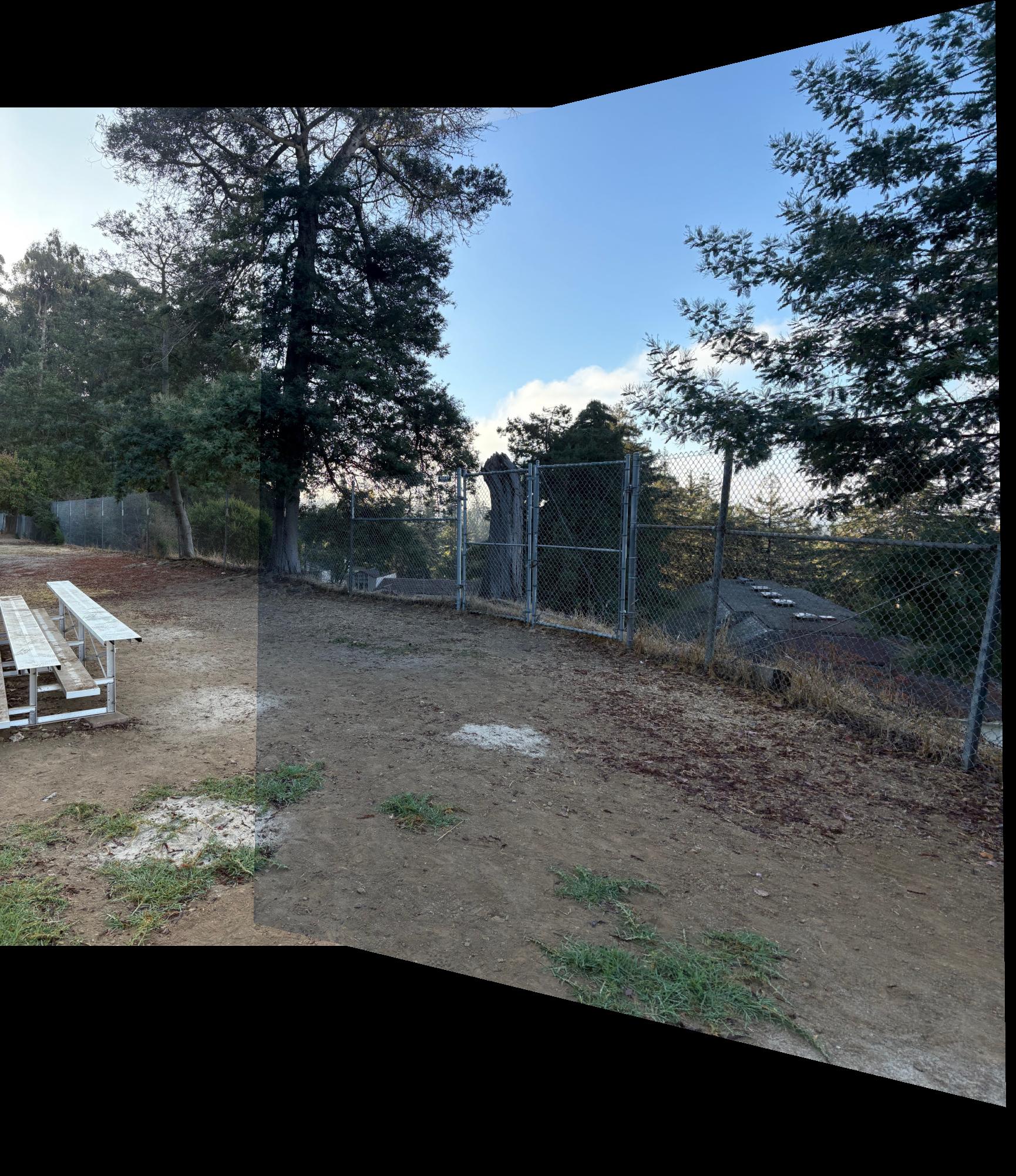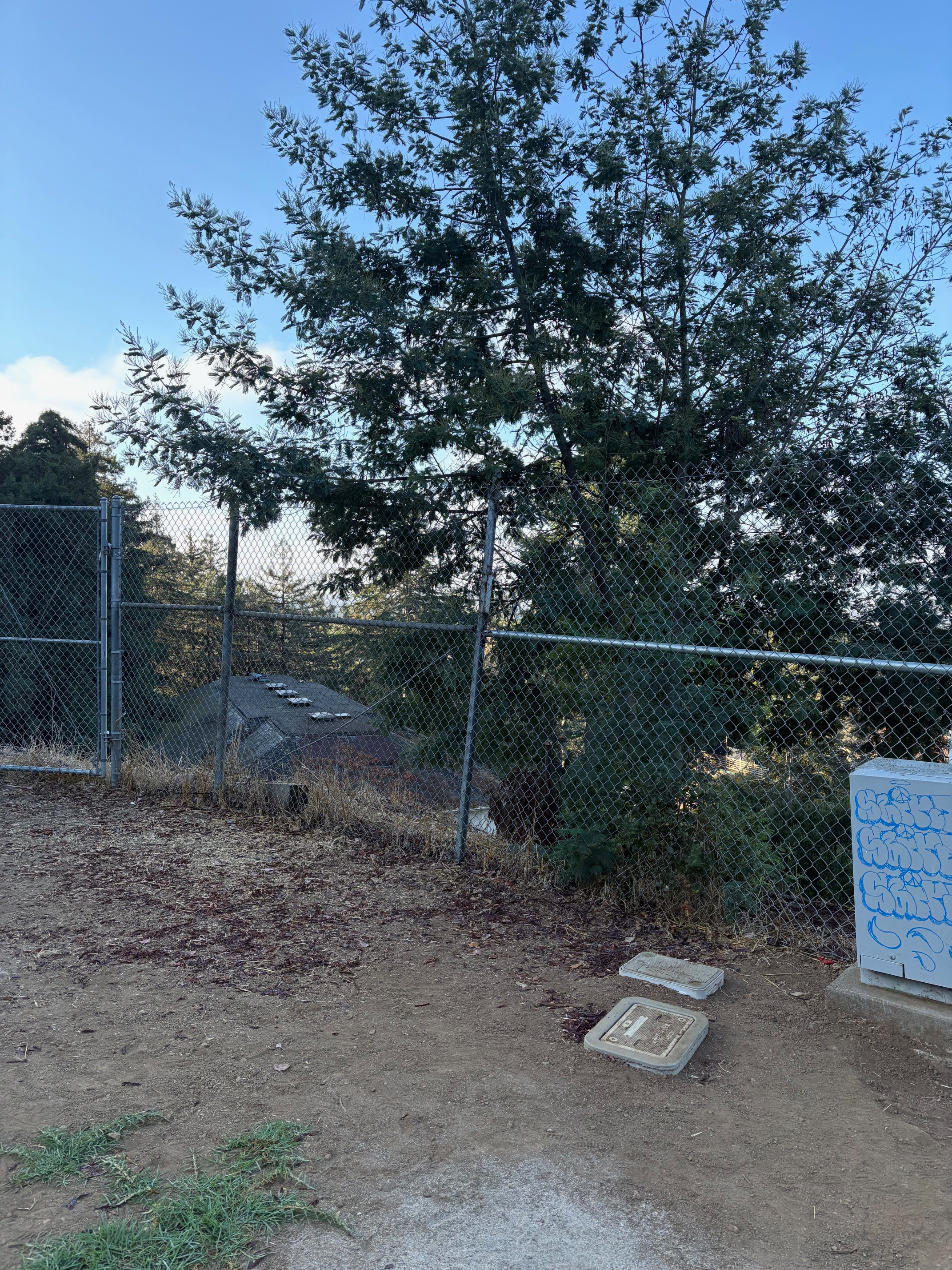Lessons Learned:

I would say the RANSAC algorithm was the most remarkable. After running RANSAC, I found correspondences that were just as good as manually labeled ones. Also, I also learned that sometimes, a convoluted passage in a research paper could be simply obscuring a relatively simpler idea.